
kang's study
3일차 : 데이터 전처리(Data preprocessing) 본문
데이터 전처리
이진 분류 binary classfication :
찾고자 하는 대상 (양성 클래스:1, 음성 클래스:0)
도미 1 빙어 0
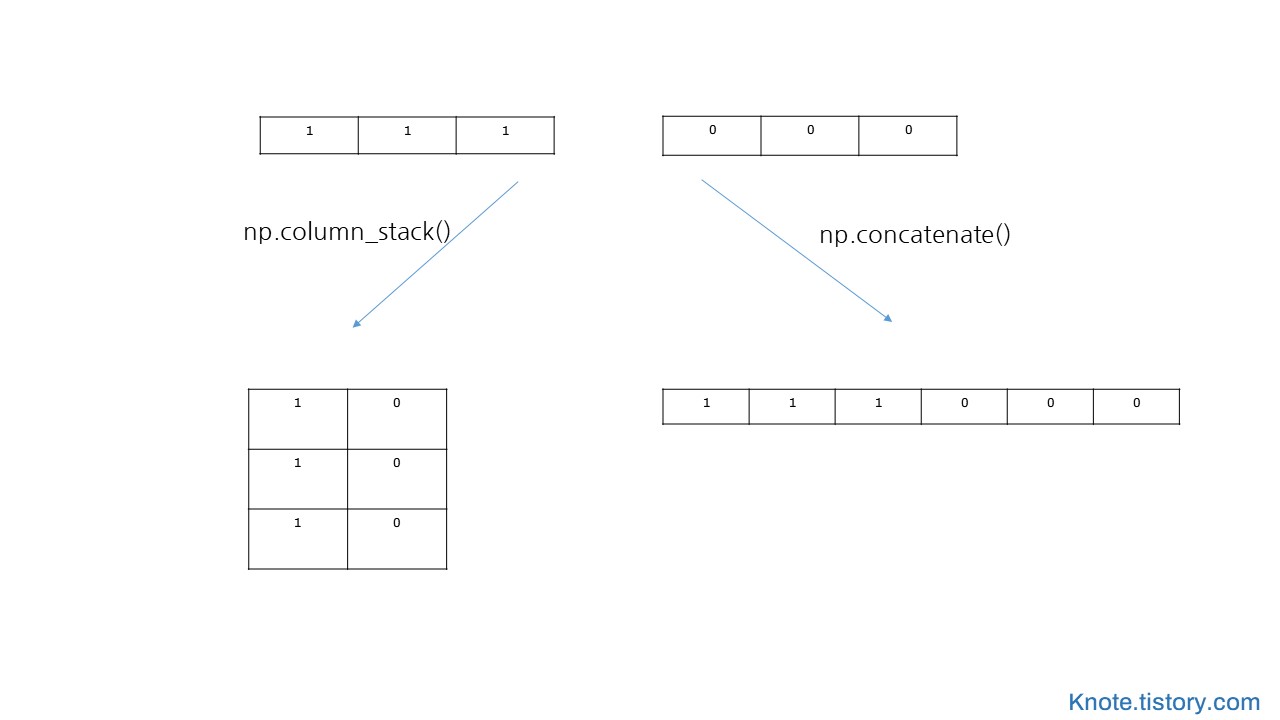
넘파이로 데이터 준비
데이터 형태
행은 샘플 열은 특성을 둔 모양을 필요로 한다.
In [ ]:
import numpy as np
In [ ]:
bream_length = [25.4, 26.3 ,26.5, 29.0, 29.0, 29.7, 29.7, 30.0, 30.0, 30.7,
                31.0, 31.0, 31.5, 32.0, 32.0, 32.0, 33.0, 33.0, 33.5, 33.5,
                34.0, 34.0, 34.5, 35.0, 35.0, 35.0, 35.0, 36.0, 36.0, 37.0,
                38.5, 38.5, 39.5, 41.0, 41.0]
bream_weight = [242.0, 290.0, 340.0, 363.0, 430.0, 450.0, 500.0, 390.0, 450.0, 500.0,
                475.0, 500.0, 500.0, 340.0, 600.0, 600.0, 700.0, 700.0, 610.0, 650.0,
                575.0, 685.0, 620.0, 680.0, 700.0, 725.0, 720.0, 714.0, 850.0, 1000.0,
                920.0, 955.0, 925.0, 972.0, 950.0]
smelt_length = [9.8, 10.5, 10.6, 11.0, 11.2, 11.3, 11.8, 11.8, 12.0, 12.2,
                12.4, 13.0, 14.3, 15.0]
smelt_weight = [6.7, 7.5, 7.0, 9.7, 9.8, 8.7, 10.0, 9.9, 9.8, 12.2,
                13.4, 12.2, 19.7, 19.9]
fish_length = bream_length + smelt_length
fish_weight = bream_weight + smelt_weight
In [ ]:
fish_data = np.column_stack((fish_length, fish_weight))
print(fish_data[0:10,:])
이전 fish_target = [1]35 + [0]14
np.ones(개수) / ((행,열)) : 개수나 행렬만큼 1으로 채움
np.zeros(개수) / ((행,열)) : 개수나 행렬만큼 0으로 채움
np.full((행,열),숫자) : 개수나 행렬만큼 원하는 숫자로 채움
In [ ]:
fish_target = np.concatenate((np.ones(35),np.zeros(14)))
print(fish_target)
사이킷런으로 데이터 나누기
In [ ]:
from sklearn.model_selection import train_test_split

train_input, test_input, train_target, test_target = train_test_split(
    fish_data, fish_target, stratify=fish_target,  random_state=42)
# stratify 값을 target으로 지정해주면 각각의 class 비율(ratio)을 train / validation에 유지해 줍니다.
# stratify는 한 쪽에 쏠려서 분배되는 것을 방지합니다
수상한 도미
In [ ]:
from sklearn.neighbors import KNeighborsClassifier
kn = KNeighborsClassifier()
kn.fit(train_input, train_target)
kn.score(test_input, test_target)
Out[ ]:
In [ ]:
print(kn.predict([[25,150]]))
In [ ]:
distances, indexes = kn.kneighbors([[25,150]]) # 이웃의 샘플 인덱스를 뽑아준다

import matplotlib.pyplot as plt

plt.scatter(train_input[:,0], train_input[:,1])
plt.scatter(25, 150, marker='^')
plt.scatter(train_input[indexes,0], train_input[indexes,1], marker='D')
plt.xlabel('length')
plt.ylabel('weight')
plt.show() # x,y의 스케일이 달라 문제가 생긴다.

거리 기반의 측정으로 데이터의 특성마다 기준이 다르면 결과가 왜곡된다.
알고리즘이 거리 기반이므로 샘플 간의 거리에 영향을 많이 받는다.
따라서 특성값을 일정한 기준으로 맞춰 주어야 한다.
In [ ]:
plt.scatter(train_input[:,0], train_input[:,1])
plt.scatter(25, 150, marker='^')
plt.scatter(train_input[indexes,0], train_input[indexes,1], marker='D')
plt.xlim((0, 1000))
plt.xlabel('length')
plt.ylabel('weight')
plt.show()
# k최근접 이웃은 스케일이 큰 특성에 영향을 많이 받는다.

표준 점수(Z점수)로 바꾸기

In [ ]:
mean = np.mean(train_input, axis=0) #axis = 0 열의 평균 , axis=1 행마다 평균
std = np.std(train_input, axis=0)

print(mean, std)

train_scaled = (train_input-mean)/std
In [ ]:
new = ([25, 150]-mean) / std # 데이터 변환은 훈련 데이터를 기준으로 한다.

plt.scatter(train_scaled[:,0], train_scaled[:,1])
plt.scatter(new[0], new[1], marker='^')
plt.xlabel('length')
plt.ylabel('weight')
plt.show()

전처리 데이터에서 모델 훈련
In [ ]:
kn.fit(train_scaled, train_target)

test_scaled = (test_input-mean) / std
# 훈련 세트를 변환한 방식 그대로 테스트 세트를 변환해야 한다.
# 훈련세트의 평균과 표준편차를 쓴다.
kn.score(test_scaled, test_target)

print(kn.predict([new]))
In [ ]:
distances, indexes = kn.kneighbors([new])

plt.scatter(train_scaled[:,0], train_scaled[:,1])
plt.scatter(new[0], new[1], marker='^')
plt.scatter(train_scaled[indexes,0], train_scaled[indexes,1], marker='D')
plt.xlabel('length')
plt.ylabel('weight')
plt.show()

출처 : 박해선, 『혼자공부하는머신러닝+딥러닝』, 한빛미디어(2021), p87-109
'[학습 공간] > [혼공머신러닝]' 카테고리의 다른 글
| 6일차 ① : 다중회귀_특성공학 (0) | 2022.03.02 |
|---|---|
| 5일차 : 선형회귀와 다항회귀 (0) | 2022.03.02 |
| 4일차 : k-최근접 이웃 회귀 (0) | 2022.03.02 |
| 2일차 : 올바른 훈련 데이터 (0) | 2022.03.02 |
| 1일차 : 머신러닝 시작 (0) | 2022.03.02 |
'[학습 공간]/[혼공머신러닝]' Related Articles
more


Comments